Google's heat map and motion chart in comparison

In addition to the motion chart (reviewed here), Google announced a heat map gadget. It's quite easy to use just like the motion chart. That is, the most difficult part is to collect data for the chart in the right format.

The following heat maps display two variables, the median age (years) and the unemployment rate (%), of countries by using colors on the world map (data source: CIA's World Factbook).

How useful is the heat map concept? Is it a good infographic?

It depends: If your target is to visualize every single variable clearly, the concept works. If your target is to help your audience understand the relationship between variables, then an XY chart works better (such as Google's motion chart--here without the animation):

Let's analyze: By average, the lower the median age is in a country, the higher the unemployment rate.

UPDATE (Thursday, April 17, 2008):

Included below a more traditional chart to display the relationship between median age and unemployment rate. In this chart, countries are grouped in median age groups. An average unemployment rate is calculated for each group.

Motion Chart provided by Google--an outstanding BI tool for free

Google just announced a gadget gallery containing one gem for the business intelligence consultants. It's a motion chart, that is, an XY chart with a time dimension (feel free to play with it).



Explanation: The XY chart above displays ten countries according to how much they collect taxes and amount of government spending (bubble size = population, bubble color = unemployment percentage). When you play years between 1970 and 1999, you see countries changing locations. By analyzing the motion it's clear that since 1970 big European countries (UK, Germany, France, Italy, Spain) have adopted policies that make them more alike (bubbles moving near each other from starting positions) while Sweden all the time stands out with high taxes and government spending. Japan seems to be the other extreme with low taxes and government spending. Between 1993 and 1997 Spain turns red with a high unemployment rate (over 20%).

I'm really astonished for several reasons:

• Motion chart as such is a very useful concept for tracking changes in time (it makes you understand the data, not just display it).
• I was able to build the chart above and publish it here in two hours, that is, very quickly as a first-time-user (+one hour more for searching useful data).
• Google motion chart works really well (try changing the chart above by using pop-up menus provided--it's a dynamic chart!).
• No else BI provider offers this kind of visualization tool.
• And it's available for free!

Of course, the motion chart concept is someting we have been waiting for ever since Google bought GapMinder. Now Google gives it for use for everybody. For example, you can load the motion chart with the products of your company and see their profiles changing over time.

Here are the steps (I made) to publish the motion chart...

1. I searched data from web with keywords "time series data". The macroeconomic data I found here. I decided to limit my test in ten countries. I collected the text data into spreadsheet. One hour.

2. The data was not in the right format for the motion chart (see example here). I used several methods to clear and pivot the data (not only in spreadsheet) until I was ready. One hour.

3. I copy-pasted the data into a Google spreadsheet document (yes, you must start using Google Docs to create and publish your motion chart). I inserted the motion chart gadget and it worked immediately. I still changed the format several times, because I needed (wanted) to learn how motion chart uses spreadsheet data. One hour.

NOTE: If you want to use quarters, months, or weeks in the time dimension, convert them into dates--such as 2008-Q3 saved as "7/1/2008" or 3rd week of 2008 saved as "1/17/2008" (Thursday, the middle day of week). Dates must be in the US format (MM/DD/YYYY) and decimal numbers with a dot as the decimal separator.

4. From the top-right gadget menu, I chose Publish Gadget, and it gave me html to put into a web page. One minute.

Final thoughts... I'm not completely satisfied with the fact that in order to use the motion chart Google will host my (perhaps confidential) data. Nevertheless I'm going to explore the motion chart concept with my customers in the future, I'm sure.

Google Chart API--why it's not important in BI?

Just for curiosity I took a look at Google Chart API. Here are two sample charts I created with it.







Nice charts. As the data and axes are controlled separately, it's possible to compose:

• A chart where axis labels are qualitative--not quantitative--which is sometimes a preferred situation in an XY chart (good vs. poor etc)
• A line chart where the line changes it's value several times within a month--not easily done in Excel or other BI tools having a direct correspondence between data values and categories displayed in the X axis

As a BI consultant, should I be interested in Google Charts?

- No. Google Chart API is a programmer tool to build larger systems.

OK. When such a larger system appears, should I be interested then?

- No again. All Google Charts are by nature static pictures (PNG files), without any means to add user interaction.

For example, if you move the mouse cursor onto a symbol (or click the symbol) in the XY chart above (or onto the line chart), nothing happens. Simply said there's no mechanism to display what the symbols represent (or what is the exact value displayed in the line chart). It's not possible to program drilling-down either. And all these features are essential in business intelligence...

Anyway, I had fun going through the Google Chart API. If you have a mind of a programmer, it's worth studying. Here are the urls which I used to create the XY chart and the line chart (broken into several lines for clarity).

• XY:
  http: //chart.apis.google.com/chart?cht=s
  &chd=s:984sttvuvkQIBLKNCAIi,DEJPgq0uov17zwopQODS,AFLPTXaflptx159gsDrn
  &chxt=x,y
  &chtt=Google+Chart+API+-+Sample+XY
  &chxl=0:Good|Poor1:Small|Large
  &chs=250x250
  &chm=o,ff000033,1,1,25
  &chg=50,50,2,5
• Line:
  http: //chart.apis.google.com/chart?cht=lc
  &chd=s:rpnpnosztwurrmmllgbZQOOORVURRSQROQSRSTKCBIKIKMLIIJIKLJKKNLNVWakiljhfedcbdcZbbZ, UVVUVVUUUVVUSSVVVXXYadfhjlmpokllmmliigdbbZZXVVUUUTU
  &chco=5555ff,ff9933
  &chtt=Google+Chart+API+-+Sample+Line
  &chls=2.0,1.0,0.0
  &chxt=x,x,y
  &chxl=0:||Oct||Nov||Dec||Jan||Feb||Mar||Apr||May||1:||2007||||||2008||||||||||2:60|70|80|90|100
  &chs=320x175
  &chg=101,25,2,5
  &chf=c,ls,0,f4f4ff,0.125,ffffff,0.125
  &chdl=First|Second

Viewing sales data by using XY charts

An XY chart (scatter plot) can express more than a typical bar or line chart. Here's an example how you can utilize typical sales data and create two interesting XY charts that help your decision making processes.

Suppose you have a typical sales table:

CREATE TABLE salesdata (
product VARCHAR(1),
customerno INTEGER,
market_area INTEGER,
day DATE,
quantity INTEGER);

.. that contains row-level sales data like this (product names A-Z, market areas 1-12):


By using the data, you usually create charts like this:



.. and for sure this chart is informative in many ways.

Now suppose you are interested in knowing more about products and market areas. For example: what is the average quantity of items sold in this season (Y), and how many of the customers bought the product for the first time (X).

You can get the data by using the two following SQL queries (this season = 2007):

/* XY for products */
SELECT s.product,
AVG(s.quantity) "Average quantity of items sold",
100*SUM(1-SIGN(ABS(s.day-q.min_day)))/COUNT(*) "% new customers in this season",
SUM(s.quantity) "Total quantity of items sold"
FROM salesdata s,
(SELECT product, customerno, MIN(day) min_day
FROM salesdata
GROUP BY product, customerno) q
WHERE s.product = q.product
AND s.customerno = q.customerno
AND s.day >= '2007-01-01'
GROUP BY s.product;

/* XY for market areas */
SELECT s.market_area,
AVG(s.quantity) "Average quantity of items sold",
100*SUM(1-SIGN(ABS(s.day-q.min_day)))/COUNT(*) "% new customers in this season",
SUM(s.quantity) "Total quantity sold in area"
FROM salesdata s,
(SELECT product, customerno, MIN(day) min_day
FROM salesdata
GROUP BY product, customerno) q
WHERE s.product = q.product
AND s.customerno = q.customerno
AND s.day >= '2007-01-01'
GROUP BY s.market_area;

Now the charts:





Let's analyze:

• Products clearly have different profiles. Product F is favored by old customers, while products L and T have recently found many new customers. In a single sales transaction, product U is sold by average nearly twice as much as D.
• Symbol size is the total quantity sold. There are no big differences in the sales of different products. More difference exist in various market areas: area 1 is the most important, while areas 9, 10, and 11 are the smallest. (I created the data by using a random function.)
• All market areas have almost the same "average quantity of items sold". The market areas differ more in X axis: in area 1 only 18% are new customers, while in areas 10 and 12 almost half of the customers are new. Perhaps the company just started marketing in areas 10 and 12?

All this is interesting -- no less so because the basic line chart cannot express this knowledge.

Nevertheless it must be said that these charts don't yet tell anything about the prospects in different market areas. Adding facts about market area size (for each product) would help your decision making where to target your marketing in the next season.

Therefore, don't be satisfied with line and bar charts, if you can improve your decision making by using XY...

Age pyramid models

In the recent days I've read with great interests Jorge Camoes' blog about his Excel Demographic Dashboard and attempts to enhance it with Crystal Xcelsius. The Excel dashboard even contains two animated reports that help you see how the age structure in various countries and continents will change between years 1995 and 2050.

First, thanks for the information! The dashboard opened my eyes to see that the trend of growing average age is valid everywhere, including African countries (not only in Europe).

Second, thanks for a good sample! This well-documented test helps us compare BI softwares against each other.

Jorge's recent post discusses different approaches to create population pyramids with Excel (XY chart) and Crystal Xcelsius (stacked bar). Excel approach appears to me more flexible, because it allows you to draw several lines (several countries) into same age pyramid. Xcelsius falls short because Xcelsius-XY chart doesn't draw lines (only data points).

Well, let me add one more approach to the age pyramid problem.



I created the four age pyramid models by using (not XY or stacked bar but) the Sheet tool in Voyant. The software allows you to format a cell (to be precise, a column of a sheet) to display a bar or a line (instead of the number it contains).

Benefits of this approach? It's the flexibility to mix numbers and graphics together. For example, if you need more space for bars or lines, numbers will immediately move to the right, because they are part of the same sheet.

OK.

From now on, a link to Jorge Camoes' BI Blog is provided under my link list.

Scatter plot found in Helsingin Sanomat

As I have criticized Helsingin Sanomat, the largest newspaper in Finland, for not publishing any scatter plot charts (XY charts), here's one!



It was published on Friday 21st September 2007 (the first XY during my blog).

The data: Number of economic reforms made (x) and economic growth rate (y) since 1989 when communism collapsed in Eastern Europe. Blue circle = European Union member state.

It's easy to see that it pays off for a state to join EU.

That's a powerful message displayed clearly. No other graph would have done that this well.

Observations about Edward Tufte's classic The Visual Display of Quantitative Information

More than two months ago I read a book The Visual Display of Quantitative Information by Edward Tufte.

Many already know this classic (1st edition 1981, 2nd 2001) that introduces the first theoretical view of statistical graphics. Instead of writing a full review, I will tell what I liked most.

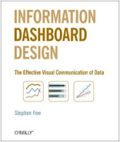
In the end of this post, you'll also find a comparison of this book and Stephen Few's Information Dashboard Design.


1. History

I enjoyed reading where all started. We don't know who invented traditional Chinese characters. We know only according to legends that the inventor of Greec alphabet was Cadmus. But for sure we know who invented line and bar charts. He was William Playfair (1759-1823). Here's one of his piece of art (its copyright has expired):



For Playfair, graphics were preferable to tables because graphics showed the shape of the data in a comparative perspective. The line chart easily contained data of hundred years displaying for example imports and exports or the national debt of Britain. Colonial wars caused rises and falls thus proving that the government policy has its economic consequences.

2. More history

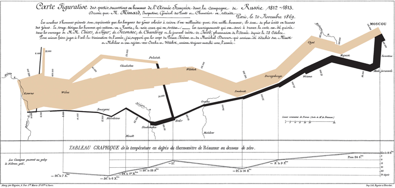
The book contains many other examples of graphical art too. As in early days every graphic was cut into metal or stone surface as a mirror image, surely each piece of graphic is more valuable and special compared to our moders graphics. Here's a masterpiece from Charles Joseph Minard (its copyright has expired):



The well-known graphic shows the terrible fate of Napoleon's army in Russia during 1812-1813. Starting from Poland on the left the size of the army is 422,000. While going towards east the width of the gray band indicates the diminishing size of the army at each place on the map. In Moscow there are 100,000 men left. Going back to Poland the dark line becomes thinner and thinner thus displaying devastating losses. In Tufte's words: It may well be the best statistical graphic ever drawn.

3. Scatterplots

Tufte uses 23 pages of 197 (11.7%) to talk about XY charts. I'm impressed about the difference he makes between XY and other charts, because I feel the same. Tufte's words: [...] the scatterplot and its variants ... [are] the greatest of all graphical designs. It links at least two variables, encouraging and even imploring the viewer to assess the possible causal relationship between the plotted variables.

In fact, when I read Helsingin Sanomat, the largest newspaper in Finland, I from time to time see it losing the possibility to use XY. The following image was published by the newspaper about the population growth rate in twenty cities of Finland (translated in English).



Here is my view of the same data by using a scatterplot:



Some cities grow fast (top-right corner) both because of natural population growth and positive net migration, while for example the lowest city Kajaani has a problem with negative net migration (-5%). A national decision-maker would appreciate this XY chart, as it clearly shows which cities are alike and which aren't.

4. Small multiples

Small multiples is something I haven't paid attention, when I was a programmer. The idea is great. See how much information is contained in the following set of charts.



Unfortunately, to create small multiples with a modern charting application is far from straightforward. For example, when composing the sample image above, I had to size and position six charts precisely to form a satisfactory result. Another bad point: Individual charts tend to have a different automatic scale in Y axis, which is a problem, when you quickly try to get grip of the data.

5. New concepts introduced

To me it's fun to learn what concepts others have invented. In this book Tufte introduces a couple of them, of which the data-ink ratio is most well-known: above all else show the data, maximize the data-ink ratio, erase non-data-ink and redundant data-ink, revise and edit.

Other concepts such as lie factor and data density I also find interesting. Lie factor: show data variation, not design variation. Data density: the small multiples chart above is an example of a high-information graphics = you don’t have to repeat titles or legends for every individual chart.

Data visualization books in comparison

As I have previously reviewed Stephen Few's Information Dashboard Design [link] that also discusses about data visualization, here's my observations how these great books differ:



By the way, there are newer books from Tufte available such as Beautiful Evidence, but I haven’t read it yet.

How to do enhanced project charts

My idea about enhanced project charting raised some discussion in the web forum provided by Perceptual Edge, Stephen Few's site.

Just to convince you it wasn't Excel (!), here's the dialog box to specify the color scale in Voyant:



Actually the process of creating such project charts in Voyant needs only three steps:

1. Create a projdata table and populate it with sample data (or use a corresponding table in your database).

CREATE TABLE projdata (
project_name VARCHAR(20),
day DATE,
hours DECIMAL(20,2));

After that it takes only 5 minutes:
2. By using a Sheet chart, specify four dimensions:

Measure: Hours = SUM(hours)
Rows: Project = project_name
Columns, outer dimension: Year = {fn YEAR({fn TIMESTAMPADD(SQL_TSI_DAY,-{fn MOD({fn DAYOFWEEK(day)}+5,7)}+3,day)})}
Columns, inner dimension: Week = {fn FLOOR(1+({fn DAYOFYEAR({fn TIMESTAMPADD(SQL_TSI_DAY,-{fn MOD({fn DAYOFWEEK(day)}+5,7)}+3,day)})}-1)/7)}

NOTE: The expressions above apply in SQL Server, MySQL, and other ODBC compatible databases. For other suitable expressions and how to limit the time frame, see my posting about monitoring changes over time.

3. Use the Sheet Cell Format dialog box (presented in the beginning): first for the whole chart, and second for the total row.

For the whole sheet, select Min & max determined automatically, so the color scale adapts to the greatest and least number of hours found from the data (excluding the total row).



For the total row, it's necessary to deselect Exclude totals, formulas, and cumulative numbers, so that the color scale adapts to the numbers presented in the total row.

It's also possible to use a tool tip to show the exact work hours by moving a mouse cursor over a cell of interest, as in the following image:



I hope we can soon see the color scale feature available in other OLAP tools too.

Viewing project data--new options available

In this posting, I will explore different ways to view project data. Some options have become available just recently.

Let's start with the well-known gantt chart. It's a great tool for project scheduling.

The gantt chart displays the start and finish date for each project. For example, the chart above shows that Project P is the longest project, starting on November 2006 finishing on August 2007.

However, a gantt chart doesn't show us how much resources each project requires.

Let's try a line chart with the same data, work hours displayed on a weekly basis.

Now we can see that project P (the longest project) doesn't require too much resources. Project K requires much more and so does A and G. You can also see the timing of these projects, that is, when the most work is done. This is important information that the gantt chart didn't tell us!

OK, let's try the area chart.

Now you can see the total resources required for all projects.

However, the line and area charts are hard to read when you have many projects. The colors of the 15 projects above are so-so distinguishable. If you have hundreds of projects, the line and area charts become useless.

Fortunately we have some new options available. Microsoft Excel calls this option "color scale" and so does Voyant's new version. Here's the same project data with Voyant.

It looks like the original gantt chart!

But instead of having just solid blue bars, now each blue bar contains much more information. First, there are weekly hours available. Second (and what is most important), the intensity of color tells us directly which project is hot and when.

If there are hundreds of projects, this kind of display still works (you just scroll down).

There's also an alternative to hide the numbers.

In the image above, the total row displays the overall resources required (red color scale).

XY chart and hierarchical graphs

Here's a video that continues the XY chart ideas in my previous postings. (Sorry for really bad blurring. Anyway, as crappy as this video is, you can see the idea.)



This sample hierarchical system (hierarchical graph) consists of 25 thousand parts in maximum eight levels. It allows me to drill-down from any branch (only one branch is open at each level). When I return to an upper level, all lower levels and nodes under it disappear and new branching starts.

Here's a better image:



This graph user interface is contextual. It's the only practical way to display large graphs in a limited space such as on a computer screen. It only shows the related nodes around the selected one. Following this principle, in a non-hierarchical graph you can display nodes linked to the central node, as well as the nodes linked to them (1st and 2nd level links). When you click a node, the clicked node becomes the central one, etc.

This kind of user interface is good for exploring large organization structures (or any hierarchical graphs). Since the system relies on the idea of drilling-down (actually, self-drilling), it's well possible to display extra information (tables and charts) about the currently selected node near the hierarchy tree (under it or to the right of it).

Technically, to calculate (x, y) coordinates, each hierarchy node has to know its level, the max number of levels, the order within its siblings (between 1...n), and the number of siblings (n).

x = my sibling id / number of siblings - 1 / (2 * number of siblings)
y = 1 - (my level / max number of levels)

The lines between nodes are drawn with the same kind of principles as in my previous postings.

XY chart and graph theory

Do you know graph theory? To me it's inspiring as such. In business intelligence, a graph (in the meaning of graph theory) provides a method to visualize relationships between entities such as between people, companies, geographical locations, etc.



Hierarchical systems, where each element of the system (except for the top element) is subordinate to a single other element, are graphs too. Various organization charts and genealogy charts (both in biology and as family trees) are good examples of such graphs.

XY chart is a good way to visualize graphs. To do it clearly, at least XY must be able to:

• Draw data points (entities)
• Draw lines between data points to visualize existing relationships
• Label data points (entities)

In my previous posting I already wrote about the first two aspects. The third aspect, labeling a data point, is necessary to understand the meaning of nodes of a graph.

The following step-by-step example shows a method how you can automatically create a graph by using XY and two tables graph_node (entities) and graph_link (relationships).

1. Create the graph_node and graph_link tables.

CREATE TABLE graph_node (node_id VARCHAR(3), node_name VARCHAR(40), node_order INTEGER, node_count INTEGER);
CREATE TABLE graph_link (node1_id VARCHAR(3), node2_id VARCHAR(3));

2. Populate tables with countries of Europe and border neighboring relationships (or anything you wish).



Note that I have included the node_order and node_count columns in the graph_node table. They are necessary to calculate (x, y) locations of data points later on. In a real situation, you should calculate node_order and node_count automatically by using SQL (or perhaps your OLAP system is able to calculate them on the fly).

By the way, there are 43 countries in Europe and 80 borders between them (not including Vatican and Turkey as nodes; including RUS-LTU, RUS-POL, and GBR-ESP relationships because of separate areas of Kaliningrad and Gibraltar).

3. Create a graph_link_view based on the two tables:

CREATE VIEW graph_link_view (link_id, datapoint_id, node_id)
AS
SELECT CONCAT(node1_id,node2_id), 0, node1_id FROM graph_link
UNION
SELECT CONCAT(node1_id,node2_id), 1, node2_id FROM graph_link
UNION
SELECT CONCAT(node1_id,node2_id), -1, NULL FROM graph_link
UNION
SELECT node_id, 0, node_id FROM graph_node
WHERE node_id not in (select node1_id from graph_link)
AND node_id not in (select node2_id from graph_link)
UNION
SELECT node_id, -1, NULL FROM graph_node
WHERE node_id not in (select node1_id from graph_link)
AND node_id not in (select node2_id from graph_link);

This view is necessary because of the way the XY chart draws data points and lines between them (see my previous posting). The following image shows some contents of the view:



Each row in graph_link table produces 3 rows in graph_link_view with datapoint_id values -1, 0, and 1 (0=start line, 1=finish line, -1=break line). Some nodes such as Iceland does not have border relationships with other country nodes, so it produces 2 rows into view (-1, 0).

4. Use the following query behind your report.

SELECT link.link_id, link.datapoint_id, node.node_id, node.node_name, node.node_order, node.node_count
FROM graph_link_view link
LEFT OUTER JOIN graph_node node ON link.node_id = node.node_id;

5. Create the measure dimension with the followin three calculations:

X = MIN(SIN(360*node.node_order/node.node_count/180*PI()))
Y = MIN(COS(360*node.node_order/node.node_count/180*PI()))
Label = MIN(node.node_id)

6. Create other dimensions as follows:

Outer category = link.link_id
Middle category = link.datapoint_id
Inner category = node.node_name (=serves as a tool tip label)

7. Create an XY chart and format it as follows:



The XY chart displays countries as data points in circle and border neighboring relationships between them as lines. Iceland and Malta aren't connected (they are islands).

A few notes:

I created this XY chart with the Voyant tool. It displays the data point label to the right of the data point. Additionally, when you move the mouse cursor over a data point, I specified the chart to display the inner category dimension as a tool tip (ISL data point displays "Iceland").

I explored some other OLAP charting tools whether or not it's possible to create the same XY. All of them seem to fall short in displaying data point labels, such as Excel, BusinessObjects Desktop Intelligence and Web Intelligence. Why such a useful feature is not supported by them, I don't know?

About the XY chart itself, it's actually somewhat hard to read, because the lines cross so often. Therefore I created another chart (below) in which I used longitudes and latitudes for (x, y) coordinates. Much better!



And of course, there's no meaning in displaying neighbor country relationships as a graph, because a simple map of Europe will do.

Nevertheless, the method above is ok to visualize connections found within customer relationship databases. For example, supposing your CRM database contains information about meetings (when, who, on which project), you can use this data to visualize which people were involved together in certain projects at certain time period. An XY graph visualizes this much better than a table.

I will now put an end to this posting, though I have two more issues in my mind:

• What to do if your graph is very large?
• Hierarchical graphs?

Later...

UPDATE (May 14, 2007): I've forgotten two borders, one between Germany and Czech Republic and another between Switzerland and Austria.

UPDATE (May 18, 2007): I recently learned that there's software for fully automated graph layout, Mathematica 6. If this functionality existed in some OLAP tool, it would be nice.

A great book about dashboard design by Stephen Few

I read a book from Stephen Few: Information Dashboard Design.

It's a great book. The idea of the book is to explain what makes business dashboards good and informative, and which mistakes we nevertheless often do and create dashboards that don't communicate.

Those of you not familiar with business dashboards I give Stephen Few's definition: A dashboard is a visual display of the most important information needed to achieve one or more objectives; consolidated and arranged on a single screen so the information can be monitored at a glange.

Why this book made me read it? Data visualization has interested me a long time. After all I was in the business for 16 years programming various graphs and making it possible to combine them in a meaningful fashion.

I liked intense discussions with my colleaques criticizing our works, which then of course have to be re-evaluated and reprogrammed, over and over again. The process inevitably increased our knowledge of data visualization. As I have now changed my job, Stephen Few's book is a mirror for me to check where my knowledge is.

Notes about the book:

The author classifies things in a nice way. For example, the dashboard categorization for various roles (strategic, analytical, and operational) made me nod my head in agreement. Yes, for sure these roles have different dashboard design challenges.

In a strategic dashboard, the big managerial picture of your business is important, budgets, actuals, and forecasts, often long terms of time (years, quarters, months), while drilling down into details is not the main issue. In an analytical dashboard, you should see everything that helps you make decisions to follow the current strategic plan, that is, by making many kind of comparisons, drilling down into details, and tracking changes in shorter terms of time (months, weeks, days). Operational dashboards are for monitoring tasks that might need action soon or right now; your interest is in intra-day periods (hours, minutes).

Classifications continue: thirteen common mistakes in dashboards (such as exceeding the boundaries of a single screen), eleven preattentive attributes of visual perception (color, position, form, motion, and their sub-categories--what works and why), the concept of data-ink ratio (eliminate unnecessary non-data pixels, enhance data pixels, highlight most important data pixels), nine graphs that communicate best (such as bar and line charts) and graphs that should be avoided (all area graphs such as pie chart, because our ability to compare 2D areas is not precise). Very thorough.

But the book is not only theory. It contains plenty of examples about good and poor dashboard design. I found amusing the idea of analyzing sample dashboards found from the web sites of software vendors (and a few other sources).

As I think this approach and myself 15 years ago starting to create samples for our OLAP charting software, what is my reaction? Yes, my first examples were poor also. The following dashboard was my invention in 1997 (the buttons on the map allow you to see weather stats of the place):



Though this is not business data, mistakes are obvious: The map takes too much space compared to data (the map here is not data but a decorative image, a simple menu or list with place names would have done better), the graphs are in wrong location (top-left is the most important region for your data, not bottom-right), too many explanatory texts (better put them into another screen and allow a user to go there by using a link), too colorful (color should be used sparingly, only to highlight what is most important or something that needs an action).

It took twelve years (!) for me to learn to design dashboards that really communicate. The following sales dashboard was my invention in 2003 (still available online here):



The idea is to start from top and see details appear in lower sections. Multiple comparisons are available (countries, customer segments, products, top 10 cities and customers, etc).

Even though I primarily designed this dashboard as a demonstration of our ideas, the model was later adopted by ProCountor, a Finnish bookkeeping agency on the web. Their customers were happy about the possibility to watch their sales accounts in a such rich way, not available in any other bookkeeping solution.

Back to the book. After showing us several design mistakes, I liked the author's bold goal to design his best dashboard models, such as the sales dashboard. Everything is put out in a communicative way, what choices he went through, etc. The resulting dashboard is versatile in ways that made me ask details from a colleague who knows sales better than I. Yes, it works.

Though a great book, I found one important area missing:

The scope of the book is non-interactive dashboards, not interactive ones. Interaction methods are not classified (the only method even mentioned is drilling-down).

As we created the Voyant OLAP tool, we included four interaction methods in it. For example, simultaneousness is an important principle in interactive dashboards. That is, in the online sales dashboard demo above (the link again here), if you choose sales "by product" in the bottom-left report, the bottom-right report is simultaneously displayed by products too.

(I hope I have time to blog about interaction methods later.)

By the way, Stephen Few writes a blog too. A link is provided here and permanently under my link list.

UPDATE (Tuesday, April 24, 2007):

After exchanging a couple of emails with the author, it appears to me that the scope of the book is on purpose limited to "non-interactive dashboards" (my term). In fact, Stephen Few kindly guided me to his article "Dashboard Confusion Revisited", available as pdf here.

In the article, he sees that "faceted analytical display" (his new term) is a different concept than "dashboard". While in a dashboard you should monitor the information at a glance, a faceted analytical display provides interaction mechanisms to reveal more perspectives (more facets) to the information.

A definition proposed by the author: A "faceted analytical display" is a set of interactive charts (primarily graphs and tables) that simultaneously reside on a single screen, each of which presents a somewhat different view of a common dataset, and is used to analyze that information.

We need these new terms and concepts to clearly talk about the issues in this growing area of knowledge!

Monitoring changes over time--my best practices

Monitoring changes over time is essential in order to make better business decisions.

Let's start with the following two graphs. (All report objects are created with the Voyant tool. Other charting tools allow you to do corresponding graphs.)



NOTE: Series A, B, C (etc) are general placeholders for your business data--they represent any phenomena compared over time such as actual vs. budget vs. forecast, sales vs. costs, revenues by operating segment or geographic region, capacity vs. actual and planned production, etc.

These simple graphs display twelve months (52 weeks) in the year chosen from the menu above the chart. Good point: the charts are simple. Bad point: you cannot easily track changes that extend to two years or more.

To enhance the charts, let's move the year dimension into the category axis.



Now you see changes over longer periods of time (good), but the graph contains too many years--11 years!--to help you easily observe changes that are happening right now (bad).

To provide more space for the category axis, you need to limit the amount of data. It's a good idea to use selection criteria such as date >= 1st January 2006. However, using a fixed date in criteria is not good--it's better to create dynamic date criteria such as date >= 1st January previous year or date >= 1st day of current month previous year. Additionally, you often want to limit dates in the future using date <= last day of the next year or something similar. Let's see how the graphs are enhanced.



As we now live April 2007 (current date printed in the bottom-right corner of the graph), it's easy to see actual and forecasted changes at a glance.

Of course it's up to your business what is the relevant period and frequency of data: previous-current-next year, last 12 months, or something else? Monthly, weekly, or daily data? Generally it's ok to watch about 50-100 data points spread on the date axis as soon as the software presents them clearly. This equals to about 8 years of monthly data, 1.5 years of weekly data, or 3 months of daily data, such as in the following image.



Nevertheless more than hundred data points are well possible, if the software provides a date axis that scales dynamically. See the following Voyant charts with 261 weekly values (5 years, each data point in Thursday) and 396 daily values (last 12+1 months)--a lot of data but very clear. The software allows you to check the exact date by moving a mouse cursor onto a line.



Technically, it depends on the database how to create dynamic date criteria and other issues discussed above. The following examples show some methods. Feel free to use and enhance them in your own projects.

In Oracle:

• Dates after first day of this year: WHERE date >= TRUNC(SYSDATE,'YYYY')
• Dates after first day of previous month: WHERE date >= TRUNC(ADD_MONTHS(SYSDATE,-1),'MM')
• Dates between previous year and next year (three years): WHERE date BETWEEN TRUNC(SYSDATE-365,'YYYY') AND TRUNC(SYSDATE+2*365,'YYYY')-1
• Dates during the last 12 months (including this month previous year): WHERE date BETWEEN TRUNC(ADD_MONTHS(SYSDATE,-12),'MM') AND TRUNC(ADD_MONTHS(SYSDATE,1),'MM')-1

In ODBC (SQL Server, MySQL, and many others):

• Dates after first day of this year: WHERE date >= {fn TIMESTAMPADD(SQL_TSI_DAY,-{fn DAYOFYEAR({fn CURDATE()})}+1, {fn CURDATE()})}
• Dates after first day of previous month: WHERE date >= {fn TIMESTAMPADD(SQL_TSI_DAY,-{fn DAYOFMONTH({fn TIMESTAMPADD(SQL_TSI_MONTH,-1,{fn CURDATE()})})}+1, {fn TIMESTAMPADD(SQL_TSI_MONTH,-1,{fn CURDATE()})})}
• Dates between previous year and next year (three years): WHERE date BETWEEN {fn TIMESTAMPADD(SQL_TSI_DAY,-{fn DAYOFYEAR({fn TIMESTAMPADD(SQL_TSI_DAY,-365,{fn CURDATE()})})}+1, {fn TIMESTAMPADD(SQL_TSI_DAY,-365,{fn CURDATE()})})} AND {fn TIMESTAMPADD(SQL_TSI_DAY,-{fn DAYOFYEAR({fn TIMESTAMPADD(SQL_TSI_DAY,2*365,{fn CURDATE()})})}, {fn TIMESTAMPADD(SQL_TSI_DAY,2*365,{fn CURDATE()})})}
• Dates during the last 12 months (including this month previous year): WHERE date BETWEEN {fn TIMESTAMPADD(SQL_TSI_DAY,-{fn DAYOFMONTH({fn TIMESTAMPADD(SQL_TSI_MONTH,-12,{fn CURDATE()})})}+1, {fn TIMESTAMPADD(SQL_TSI_MONTH,-12,{fn CURDATE()})})} AND {fn TIMESTAMPADD(SQL_TSI_DAY,-{fn DAYOFMONTH({fn TIMESTAMPADD(SQL_TSI_MONTH,1,{fn CURDATE()})})}+1, {fn TIMESTAMPADD(SQL_TSI_MONTH,1,{fn CURDATE()})})}

You also need expressions to create years, months, weeks, etc.

In Oracle:

• Year: TO_NUMBER(TO_CHAR(date,'YYYY'))
• Month: TO_NUMBER(TO_CHAR(date,'MM'))
• Year (when used with ISO standard week): TO_NUMBER(TO_CHAR(date,'IYYY'))
• Week, ISO standard starting on Monday: TO_NUMBER(TO_CHAR(date,'IW'))
• Day of month: TO_NUMBER(TO_CHAR(date,'DD'))
• Date as such: date
• Week (as a date value of Thursday = the middle day of week): date-TO_NUMBER(TO_CHAR(date,'D'))+4

In ODBC (SQL Server, MySQL, and many others):

• Year: {fn YEAR(date)}
• Month: {fn MONTH(date)}
• Year (when used with ISO standard week): {fn YEAR({fn TIMESTAMPADD(SQL_TSI_DAY,-{fn MOD({fn DAYOFWEEK(date)}+5,7)}+3,date)})}
• Week, ISO standard starting on Monday: {fn FLOOR(1+({fn DAYOFYEAR({fn TIMESTAMPADD(SQL_TSI_DAY,-{fn MOD({fn DAYOFWEEK(date)}+5,7)}+3,date)})}-1)/7)}
• Day of month: {fn DAYOFMONTH(date)}
• Date as such: date
• Week (as a date value of Thursday = the middle day of week): {fn TIMESTAMPADD(SQL_TSI_DAY,-{fn MOD({fn DAYOFWEEK(date)}+5,7)}+3,date)}

Happy charting :)

Red sunsets and air quality--what chart to use?

Spring is two weeks early in Southern Finland. Ice and snow has melted, brooks and rivers are full of water, birds migrate north over the Gulf of Finland, and sunsets are beautiful reddish.

Red sunsets? They might please the eye, but also make my eyes itch when riding my bike. The red color is in fact caused by numerous air pollutants: small particles released from snow and spread all over by traffic, also from burning branches and trees. I'm waiting a heavy rain to wash the dust away.

(Aside: The Japanese flag represents the rising red sun, probably designed thousand years ago. Did the designer live in a village where people burned a lot of tree in wintertime? Did he or she understand our modern age will see in the flag a proof of air pollution?)

I'm slowly getting towards my point, data visualization, one of my key interests :)

Since the air quality is a worry to people nowadays, the largest newspaper in Finland, Helsingin Sanomat, published the following chart a few days ago.

Air quality in three different places during recent five days

Is the data output well designed? Not at all.

When air quality is good, bars are short; when bad, long. Yep. I'm able to get the information but still, the BAR CHART makes me ask in what sense bad air should be "longer" or "more" than good air?

Another thing, there are colored bands in the background to tell the air quality in words: good, satisfactory, so-so, bad, very bad. The bands for satisfactory and so-so are narrower than good and bad, while very bad is a much wider band than others. Why? Does that carry some message I should understand?

A probable explanation: The graphic designer gets exact figures of air pollutant concentrations every day. Color bands are concentration ranges defined by health care authorities. When drawing the chart, the designer hides exact numbers and adds color bands to correspond the good, satisfactory, so-so, etc air quality ranges.

But we humans don't think like this!

To us the air quality is either good or bad (or something between the opposites) without having to think which extreme is "more" and which is "less". The scale is irrelevant as soon as you can understand changes over time.

Below is my proposition how the newspaper should do it (the data is partially my imagination such as forecasted rains starting tomorrow).

In this presentation of two charts, air quality is no more a separate phenomenon but comparable to temperature and precipitation (which indeed influence the air quality). A line chart displays changes in air quality clearly. A longer period helps readers put the current air quality in context.

Much better than the original, don't you think?

How about you? Do you also share the same passion to enhance charts and tables printed in daily papers? :)

Hello world

While I soon start to work in Affecto, one of the largest business intelligence companies in Northern Europe, it's a good moment to start blogging about BI.

About my background, I have 16 years of history in business intelligence. All these years I've been in the developer side, creating an OLAP tool Voyant. I'm proud to tell that the software has been appreciated by customers for its ease of use and productivity, nevertheless it has not gained a big success.

Data visualization is one of my key interests, so my goal is to include an image or two in every posting. The next one is a dashboard I once made to express Voyant's elegant customizable web interface (click here for an online web demo).



For those of you being technically interested, Voyant relies on lightweight Java applets in the browser environment (three applets in the example above). The Server version delivers data between database and applets. The Designer and Analyst desktop versions are for specifying report objects and their interaction.

Outside of data visualization (and Voyant), I'll plan to write about good and bad sides of those OLAP/BI tools I'll be working with as a consultant during the following months.

I hope my BI background will help me see and write about business intelligence in a fresh way.